Un-stack Data / Row to column [QSS Series]

    Welcome to 1st post of QSS where we will see how to un-stack data or convert range of column in to multiple rows. so without wasting much time let's jump on to it.

[QSS] Unstack Data / Row to column

Problem

Solution

I hope you love it and use it as and when required.

Love to hear you in comment.

QSS Series - Quick and Smart Solution Series

Hello Guys,

I am back after almost 3 month. After getting an overwhelming response from excel communities and other visitors, I am coming up with new series on this blog named QSS (Quick & Smart Solution). in this QSS Series, Post on this blog will not eat much of your research time and directly focus on quick and smart solution of said problem in excel.

You can simply search for QSS in search box on blog and get list of all Quick and Smart Solution posts.

in upcoming time, i will also add QSS (Quick & Smart Solution) page where you can get one stop solution of all tiny to big excel problems.

As usual i would like to receive issues and suggestion on GyanOfExcel@Gmail.com

Thank you again for visiting. 

Add Time and Date Stamp in Data Entry Automatically in Excel

 Now a days, Data entry is not remained isolated job but that is now become necessary for many type of data related work like record keeping or database management or other data entry related job.

    Time of entry of such record become very important part for analysis and research. in excel as such there is no feature to maintain Time and date stamp of entry done in particular cell. So in this post, we will try to learn how to put simple IF and NOW function to get Date and Time do data entered in particular cell.

First do the below quick setting to make it working.

Follow below steps to learn how it is working. 

I hope you enjoyed it and next time you will use it.

SUBTOTAL Formula in Excel for Filtered Data / Table. (SUBTOTAL is not only TOTAL, but more of it)

    In Excel, We can filter data as we need by selecting criteria. sometime we need to do some calculation on that filtered data. SUBTOTAL formula can help you in that.

First we will understand how to use SUBTOTAL formula by selecting various function according to your need in data.

Function List:

Function	Number
AVERAGE	1 or 101
COUNT	2 or 102
COUNTA	3 or 103
MAX	4 or 104
MIN	5 or 105
PRODUCT	6 or 106
STDV	7 or 107
STDEVP	8 or 108
SUM	9 or 109
VAR	10 or 110

Now, you are ready with formula. in below step you will see the real usage of this formula.

SUBTOTAL do the calculation on visible / filtered data only.

You can make it more advance by using slicer on your data.

(No need to worry if you dont know slicer or table, Just CLICK HERE)

I hope you find this useful and will you this tomorrow in your office.

Pivot Table and Slicer in Excel

In Excel, A Pivot Table is a table of summary of massive or big data table. In this summary you can include sums, averages, or other statistics, which the pivot table groups together in a meaningful way.

Let's learn it in below steps...

1. How to Insert Pivot table in excel

(Click on Image to see)

2. How to add Rows and Columns in Pivot table

(Click on Image to see)

3. How to insert Slicer in Pivot table

(Click on image to see)

4. How to turn cell range into table and use slicer on it.

(Click on image to see)

5. How to use Slicer for Dynamic Chart.

(Click on image to see)

6. How to change Pivot Table Layout.

(Click on image to see)

I hope you have learn to use Table, Pivot Table and Slicer to make dynamic data in Excel.

Daily useful Excel FORMULA

There are many small and day to day useful formula in excel for smart solutions. below are the list of them. more are coming soon...

(Click on Image to see)

Comment which one you like the most.

Useful Excel Shortcut and Short hands

Below are useful and handy excel shortcut which can save your time by regularly practicing it while working on Excel.

Short hands: You have to press keys one by one, not together.

ALT  O  C  A    =    Auto fit Row with content

ALT  H  A  C    =    Central Align in cell

ALT  H  B  A    =    Apply All Border in selected cell

ALT  H  B  N    =    Remove All Border in selected cell

ALT  H  M  M    =    Merge selected cell

ALT  H  A  C    =    Central Align in cell

ALT H V V       =    Paste as Value

F4                    =     Lock row or column in formula

F12                  =    Open Save As dialogue box

F7                    =     Spell check

F2                    =      Edit selected cell

Shortcuts: You have to press keys together.

CTRL  D         =    Copy content from above cell

CTRL  R         =    Copy content from right side cell

CTRL SHIFT L =   Apply / Remove filter in selected row

CTRL 1          =     Format cell window

CTRL  F        =      Find window

CTRL H        =       Replace window

CTRL PGUP or PGDN = Switching between sheets

CTRL Arrow key  = Go to last cell of data or Table

CTRL Shift Arrow key  = Select upto last cell of data or Table

Shift Space   =        Select Row

CTRL Space   =      Select Column

ALT    =            =    Auto sum

CTRL  T            =   Convert Range into Table

CTRL  ;            =   Insert today's date

CTRL SHIFT  ; = Insert Time

Which Shortcut you like the most? share in comment.

Combine VLOOKUP and MATCH formula and see the MAGIC !!!

    

    In previous post, we have learnt how to use VLOOKUP, but when you are required to fight with massive data with lots of columns and row then it will be time consume to use VLOOKUP.

But in that case, when we add one more small formula in VLOOKUP, It will work like professional database management software, and the ingredient is MATCH formula. You wonder how?  its very easy and can be done in two below steps.

Step. 1

(Click on Image to see)

Step. 2

(Click on Image to see)

Working smooth? Great.

Learn VLOOKUP in 40 Seconds in excel

In Excel, sometime we need to fetch data from table with some criteria. for that you can use many methods. Vlookup is one of the most popular of them.

In this post, we will learn Vlookup in just less than minute by following image.

(Click on Image to see)

Usage of Excel Status bar instead of basic formulas

Hello Friends,

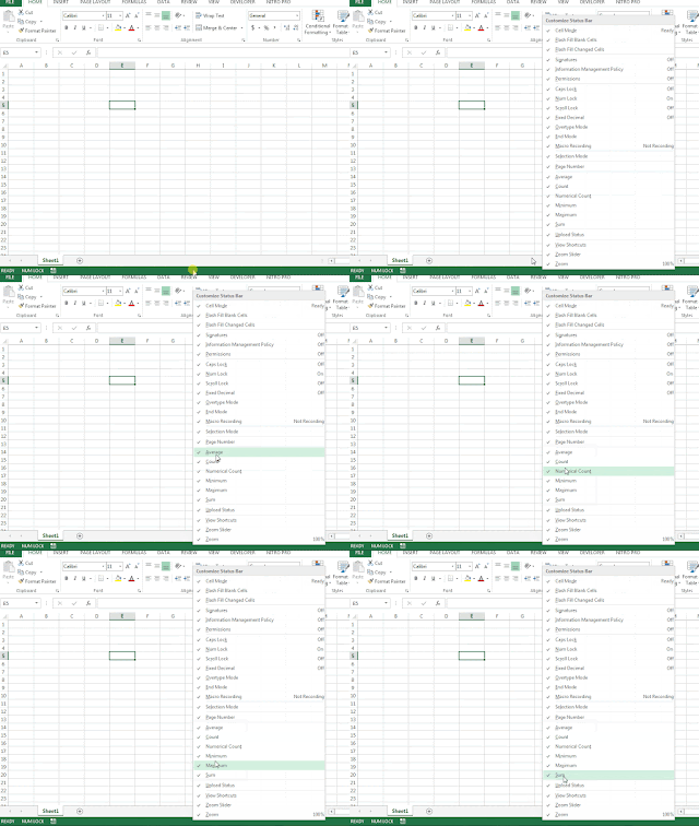
    Welcome to Gyaan of Excel. Many a times in excel, we need to have quick look on our data or number's sum or average or count or minimum or maximum value without putting much efforts or formula on sheet. we can do it it quickly by following simple steps.

1. Right click on excel status bar and check all shown options

(Click on Image to see)

2. Just by selecting data in you sheet you can see all the calculation on bottom status bar.

(Click on Image to see)

I hope you like this small and silly trick of excel. stay tuned and keep learning with Gyaan of Excel.